mastR: Simplified Customized Design For Differential Expression Analysis
Jinjin Chen
Bioinformatics Division, Walter and Eliza Hall Institute of Medical Research, Parkville, VIC 3052, AustraliaDepartment of Medical Biology, University of Melbourne, Parkville, VIC 3010, Australiachen.j@wehi.edu.au
Ahmed Mohamed
Bioinformatics Division, Walter and Eliza Hall Institute of Medical Research, Parkville, VIC 3052, Australiamohamed.a@wehi.edu.au
Chin Wee Tan
Bioinformatics Division, Walter and Eliza Hall Institute of Medical Research, Parkville, VIC 3052, Australiacwtan@wehi.edu.au
20 May 2026
Source:vignettes/mastR_customized_design.Rmd
mastR_customized_design.RmdIntroduction
Simplified Customized Design For Differential Expression Analysis
mastR provides a simplified customized contrast design
for differential expression analysis, which can help users handle the
complex experimental design and data structure in one simple function
call.
The function process_data() in mastR allows
users to pass a customized contrast matrix to the function, which can
give users more flexibility.
Installation
mastR R package can be installed from Bioconductor or GitHub.
The most updated version of mastR is hosted on GitHub
and can be installed using devtools::install_github()
function provided by devtools.
# if (!requireNamespace("devtools", quietly = TRUE)) {
#   install.packages("devtools")
# }
# if (!requireNamespace("mastR", quietly = TRUE)) {
#   devtools::install_github("DavisLaboratory/mastR")
# }

if (!requireNamespace("BiocManager", quietly = TRUE)) {
  install.packages("BiocManager")
}
if (!requireNamespace("mastR", quietly = TRUE)) {
  BiocManager::install("mastR")
}
packages <- c(
  "BiocStyle",
  "clusterProfiler",
  "ComplexHeatmap",
  "depmap",
  "enrichplot",
  "ggrepel",
  "Glimma",
  "gridExtra",
  "jsonlite",
  "knitr",
  "rmarkdown",
  "RobustRankAggreg",
  "rvest",
  "singscore",
  "UpSetR"
)
for (i in packages) {
  if (!requireNamespace(i, quietly = TRUE)) {
    install.packages(i)
  }
  if (!requireNamespace(i, quietly = TRUE)) {
    BiocManager::install(i)
  }
}Example
Here we use the example data im_data_6 from GSE60424
(Download using GEOquery::getGEO()), consisting of immune
cells from healthy individuals.
im_data_6 is a eSet object, containing
RNA-seq TMM normalized counts data of 6 sorted immune cell types each
with 4 samples. More details in ?mastR::im_data_6.
data("im_data_6")
im_data_6
#> ExpressionSet (storageMode: lockedEnvironment)
#> assayData: 50045 features, 24 samples
#>   element names: exprs
#> protocolData: none
#> phenoData
#>   sampleNames: GSM1479438 GSM1479439 ... GSM1479525 (24 total)
#>   varLabels: title geo_accession ... years since diagnosis:ch1 (66
#>     total)
#>   varMetadata: labelDescription
#> featureData: none
#> experimentData: use 'experimentData(object)'
#>   pubMedIds: 25314013
#> Annotation: GPL15456
1. Customized contrast matrix
The customized contrast matrix can be created using
makeContrasts() function from limma
package.
Users can create the customized contrast matrix manually by specifying the contrast names and the levels of the groups.
## DE of NK vs B and B vs T
con_mat <- makeContrasts(
  'NK-CD4' = 'NK - CD4',
  'NK-T' = 'NK - (CD4 + CD8)/2',
  levels = levels(factor(make.names(im_data_6$`celltype:ch1`)))
)
con_mat
#>              Contrasts
#> Levels        NK-CD4 NK-T
#>   B.cells          0  0.0
#>   CD4             -1 -0.5
#>   CD8              0 -0.5
#>   Monocytes        0  0.0
#>   Neutrophils      0  0.0
#>   NK               1  1.0
However, it is important to note that the levels of the groups should be consistent with the levels of the groups in the expression matrix. Otherwise, the contrast matrix will not be correct and the analysis will stop with an error.
So it is recommended and safer to create the customized contrast
matrix from the design matrix generated from process_data()
function.
What we need to do is to first process the data using
process_data() function with random target group, then
extract the design matrix from the proc_data object.
Next, we can create the customized contrast matrix from the design matrix.
proc_data <- mastR::process_data(
  im_data_6,
  group_col = 'celltype:ch1',
  target_group = 'NK',
  summary = FALSE,
  gene_id = "ENSEMBL" ## rownames of im_data_6 is ENSEMBL ID
)
con_mat2 <- makeContrasts(
  'NK-CD4' = 'NK - CD4',
  'NK-T' = 'NK - (CD4 + CD8)/2',
  levels = proc_data$vfit$design
)
con_mat2
#>              Contrasts
#> Levels        NK-CD4 NK-T
#>   B.cells          0  0.0
#>   CD4             -1 -0.5
#>   CD8              0 -0.5
#>   Monocytes        0  0.0
#>   Neutrophils      0  0.0
#>   NK               1  1.0

identical(con_mat, con_mat2)
#> [1] TRUE
2. Process data
Then, we can use the process_data() function to obtain
the DE results with the customized contrast design.
At this point, the DE analysis is performed based on the customized contrast design, regardless of the target group.
proc_data <- mastR::process_data(
  im_data_6,
  group_col = 'celltype:ch1',
  target_group = 'NK',
  contrast_mat = con_mat, ## specify contrast of NK vs B and B vs T
  summary = TRUE,
  gene_id = "ENSEMBL" ## rownames of im_data_6 is ENSEMBL ID
)
#>        NK-CD4 NK-T
#> Down     2694 2678
#> NotSig   4985 4935
#> Up       2732 2798

## plot mean-var
mastR::plot_mean_var(proc_data)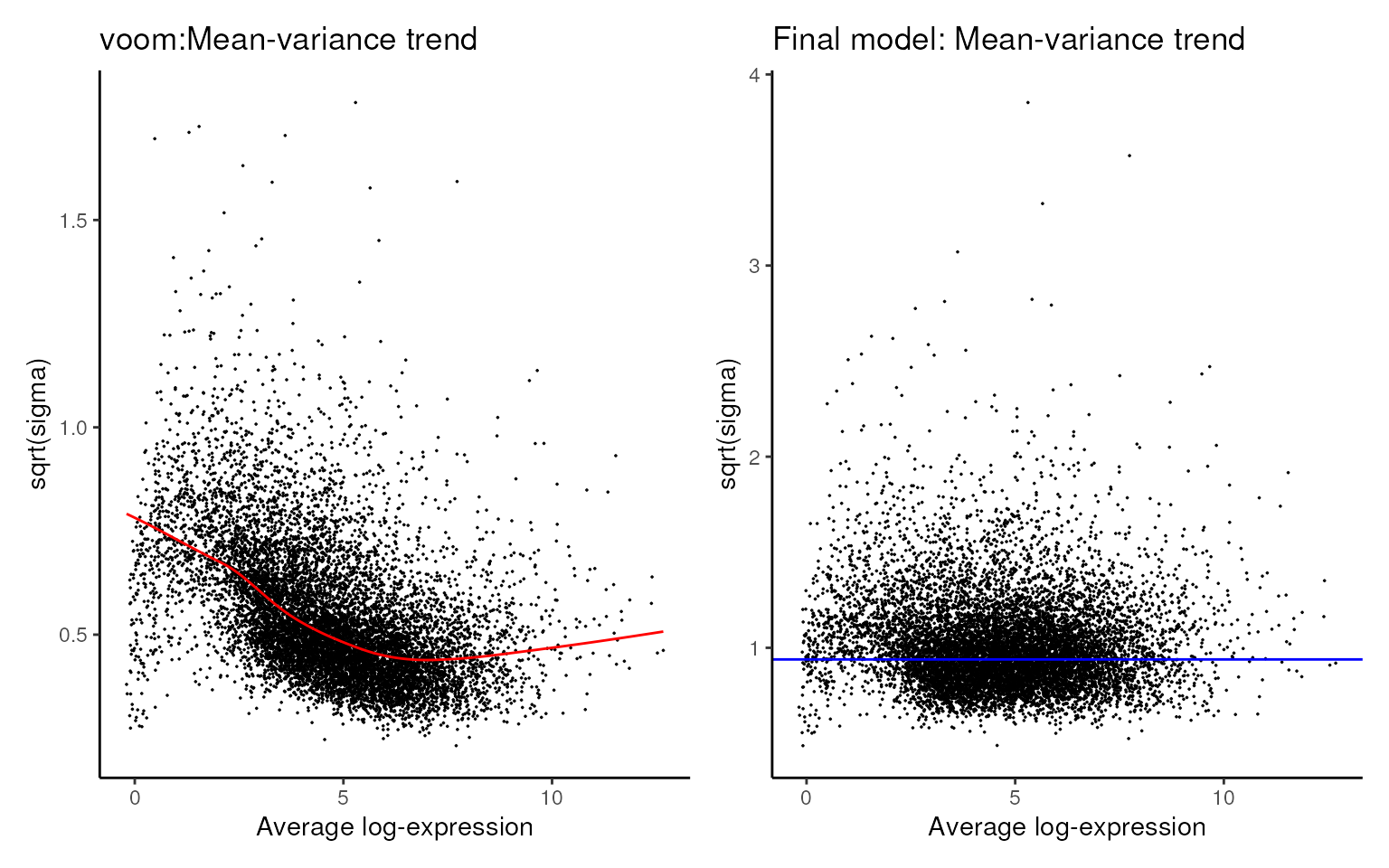
3. Results
The DE results are stored in the proc_data object and
can be easily accessed via proc_data$tfit.
## contrast names
colnames(proc_data$tfit)
#> [1] "NK-CD4" "NK-T"

## DE results for 'NK-B' contrast
na.omit(limma::topTreat(
  proc_data$tfit,
  coef = 1, # or 'NK-B' for the first contrast
  number = Inf # get all DE results
)) |> head()
#>                     logFC  AveExpr         t      P.Value    adj.P.Val
#> ENSG00000229164 -5.277165 3.816770 -27.57282 1.573629e-18 9.709102e-15
#> ENSG00000167286 -5.685866 2.309187 -26.96013 2.542590e-18 9.709102e-15
#> ENSG00000137078 -5.862098 1.745241 -26.77409 2.947367e-18 9.709102e-15
#> ENSG00000172673 -6.209083 1.783905 -26.29011 4.348395e-18 9.709102e-15
#> ENSG00000160185 -6.268015 1.707258 -26.20408 4.662906e-18 9.709102e-15
#> ENSG00000065357 -3.492239 7.339261 -25.51861 8.197948e-18 1.422481e-14
Of course, users can also use the get_de_table()
function to easily get all DE result tables for all contrasts on a
single call.
## DE results for all contrasts
DE_table <- mastR::get_de_table(
  im_data_6,
  group_col = 'celltype:ch1',
  target_group = 'NK',
  contrast_mat = con_mat, ## specify contrast of NK vs B and B vs T
  summary = TRUE,
  gene_id = "ENSEMBL" ## rownames of im_data_6 is ENSEMBL ID
)
#>        NK-CD4 NK-T
#> Down     2694 2678
#> NotSig   4985 4935
#> Up       2732 2798
names(DE_table)
#> [1] "NK-CD4" "NK-T"

head(DE_table[[1]])
#>                     logFC  AveExpr         t      P.Value    adj.P.Val
#> ENSG00000229164 -5.277165 3.816770 -27.57282 1.573629e-18 9.709102e-15
#> ENSG00000167286 -5.685866 2.309187 -26.96013 2.542590e-18 9.709102e-15
#> ENSG00000137078 -5.862098 1.745241 -26.77409 2.947367e-18 9.709102e-15
#> ENSG00000172673 -6.209083 1.783905 -26.29011 4.348395e-18 9.709102e-15
#> ENSG00000160185 -6.268015 1.707258 -26.20408 4.662906e-18 9.709102e-15
#> ENSG00000065357 -3.492239 7.339261 -25.51861 8.197948e-18 1.422481e-14
Visualization
Users can use the glimmaMDS(), glimmaMA(),
and glimmaVolcano() functions from Glimma
package to visualize the data and DE results interactively.
## MDS plot
Glimma::glimmaMDS(proc_data)

## MA plot
Glimma::glimmaMA(proc_data$tfit, dge = proc_data)

## volcano plot
Glimma::glimmaVolcano(proc_data$tfit, dge = proc_data)
Session Info
sessionInfo()
#> R version 4.3.3 (2024-02-29)
#> Platform: x86_64-pc-linux-gnu (64-bit)
#> Running under: Ubuntu 22.04.4 LTS
#>
#> Matrix products: default
#> BLAS:   /usr/lib/x86_64-linux-gnu/openblas-pthread/libblas.so.3
#> LAPACK: /usr/lib/x86_64-linux-gnu/openblas-pthread/libopenblasp-r0.3.20.so;  LAPACK version 3.10.0
#>
#> locale:
#>  [1] LC_CTYPE=en_US.UTF-8       LC_NUMERIC=C
#>  [3] LC_TIME=en_US.UTF-8        LC_COLLATE=en_US.UTF-8
#>  [5] LC_MONETARY=en_US.UTF-8    LC_MESSAGES=en_US.UTF-8
#>  [7] LC_PAPER=en_US.UTF-8       LC_NAME=C
#>  [9] LC_ADDRESS=C               LC_TELEPHONE=C
#> [11] LC_MEASUREMENT=en_US.UTF-8 LC_IDENTIFICATION=C
#>
#> time zone: UTC
#> tzcode source: system (glibc)
#>
#> attached base packages:
#> [1] stats4    stats     graphics  grDevices utils     datasets  methods
#> [8] base
#>
#> other attached packages:
#>  [1] GSEABase_1.64.0      graph_1.80.0         annotate_1.80.0
#>  [4] XML_3.99-0.16.1      AnnotationDbi_1.64.1 IRanges_2.36.0
#>  [7] S4Vectors_0.40.2     Biobase_2.62.0       BiocGenerics_0.48.1
#> [10] ggplot2_3.5.0        edgeR_4.0.16         limma_3.58.1
#> [13] mastR_1.13.1         BiocStyle_2.30.0
#>
#> loaded via a namespace (and not attached):
#>   [1] DBI_1.2.2                   bitops_1.0-7
#>   [3] rlang_1.1.3                 magrittr_2.0.3
#>   [5] matrixStats_1.3.0           compiler_4.3.3
#>   [7] RSQLite_2.3.6               png_0.1-8
#>   [9] systemfonts_1.0.6           vctrs_0.6.5
#>  [11] pkgconfig_2.0.3             crayon_1.5.2
#>  [13] fastmap_1.1.1               backports_1.4.1
#>  [15] XVector_0.42.0              labeling_0.4.3
#>  [17] utf8_1.2.4                  rmarkdown_2.26
#>  [19] ragg_1.3.0                  purrr_1.0.2
#>  [21] bit_4.0.5                   xfun_0.43
#>  [23] zlibbioc_1.48.2             cachem_1.0.8
#>  [25] GenomeInfoDb_1.38.8         jsonlite_1.8.8
#>  [27] blob_1.2.4                  highr_0.10
#>  [29] DelayedArray_0.28.0         broom_1.0.5
#>  [31] parallel_4.3.3              R6_2.5.1
#>  [33] bslib_0.7.0                 parallelly_1.37.1
#>  [35] car_3.1-2                   GenomicRanges_1.54.1
#>  [37] jquerylib_0.1.4             SummarizedExperiment_1.32.0
#>  [39] Rcpp_1.0.12                 bookdown_0.39
#>  [41] knitr_1.46                  future.apply_1.11.2
#>  [43] Matrix_1.6-5                tidyselect_1.2.1
#>  [45] abind_1.4-5                 yaml_2.3.8
#>  [47] codetools_0.2-20            listenv_0.9.1
#>  [49] lattice_0.22-6              tibble_3.2.1
#>  [51] withr_3.0.0                 KEGGREST_1.42.0
#>  [53] evaluate_0.23               future_1.33.2
#>  [55] desc_1.4.3                  Biostrings_2.70.3
#>  [57] pillar_1.9.0                BiocManager_1.30.22
#>  [59] ggpubr_0.6.0                MatrixGenerics_1.14.0
#>  [61] carData_3.0-5               generics_0.1.3
#>  [63] sp_2.1-3                    RCurl_1.98-1.14
#>  [65] munsell_0.5.1               scales_1.3.0
#>  [67] globals_0.16.3              xtable_1.8-4
#>  [69] glue_1.7.0                  tools_4.3.3
#>  [71] locfit_1.5-9.9              ggsignif_0.6.4
#>  [73] dotCall64_1.1-1             fs_1.6.3
#>  [75] grid_4.3.3                  tidyr_1.3.1
#>  [77] SingleCellExperiment_1.24.0 colorspace_2.1-0
#>  [79] GenomeInfoDbData_1.2.11     patchwork_1.2.0
#>  [81] msigdb_1.10.0               cli_3.6.2
#>  [83] textshaping_0.3.7           spam_2.10-0
#>  [85] fansi_1.0.6                 S4Arrays_1.2.1
#>  [87] dplyr_1.1.4                 gtable_0.3.5
#>  [89] rstatix_0.7.2               sass_0.4.9
#>  [91] digest_0.6.35               progressr_0.14.0
#>  [93] SparseArray_1.2.4           farver_2.1.1
#>  [95] org.Hs.eg.db_3.18.0         htmlwidgets_1.6.4
#>  [97] SeuratObject_5.0.1          memoise_2.0.1
#>  [99] htmltools_0.5.8.1           pkgdown_2.0.9
#> [101] lifecycle_1.0.4             httr_1.4.7
#> [103] statmod_1.5.0               bit64_4.0.5