A quick start guide to smartid: Scoring and MARker selection method based on modified Tf-IDf

Introduction

smartid

smartid is a package that enables automated selection of group specific signature genes, especially for rare population. This package is developed for generating lists of specific signature genes based on Term Frequency-Inverse Document Frequency (TF-IDF) modified methods and expectation maximization (EM) for labeled data. It can also be used as a new gene-set scoring method or data transformation method for un-labeled data. Multiple visualization functions are implemented in this package.

Installation

smartid R package can be installed from Bioconductor or GitHub.

The most updated version of smartid is hosted on GitHub and can be installed using devtools::install_github() function provided by devtools.

if (!requireNamespace("BiocManager", quietly = TRUE)) {
  install.packages("BiocManager")
}
if (!requireNamespace("smartid", quietly = TRUE)) {
  BiocManager::install("smartid")
}

Prepare Data

To show a quick start guide of smartid, here we use package splatter to simulate a scRNA-seq data of 1000 genes * 3000 cells. This data consists of 4 groups, each has 2% DEGs except Group 4, which has no DEG as a negative control group.

library(smartid)
library(SummarizedExperiment)
library(splatter)
library(ggplot2)
library(scater)

## set seed for reproducibility
set.seed(123)
sim_params <- newSplatParams(
  nGenes = 1000,
  batchCells = 3000,
  group.prob = seq(0.1, 0.4, length.out = 4),
  de.prob = c(0.02, 0.02, 0.02, 0),
  # de.downProb = 0,
  de.facLoc = 0.5,
  de.facScale = 0.4
)

data_sim <- splatSimulate(sim_params, method = "groups")

## get up markers based on fold change
fc <- 1
cols <- paste0("DEFacGroup", seq_along(unique(data_sim$Group)))
defac <- as.data.frame(rowData(data_sim)[, cols])
up <- lapply(cols, \(id)
dplyr::filter(defac, if_all(-!!sym(id), \(x) !!sym(id) / x > fc)) |>
  rownames())
slot(data_sim, "metadata")$up_markers <- setNames(up, cols)
slot(data_sim, "metadata")$up_markers
#> $DEFacGroup1
#>  [1] "Gene31"  "Gene42"  "Gene172" "Gene225" "Gene308" "Gene312" "Gene352"
#>  [8] "Gene391" "Gene425" "Gene436" "Gene547" "Gene650" "Gene696" "Gene893"
#> [15] "Gene904" "Gene913"
#> 
#> $DEFacGroup2
#>  [1] "Gene37"  "Gene76"  "Gene141" "Gene332" "Gene419" "Gene628" "Gene682"
#>  [8] "Gene713" "Gene778" "Gene818"
#> 
#> $DEFacGroup3
#> [1] "Gene26"  "Gene28"  "Gene357" "Gene405" "Gene462" "Gene518" "Gene833"
#> 
#> $DEFacGroup4
#> character(0)
data_sim
#> class: SingleCellExperiment 
#> dim: 1000 3000 
#> metadata(2): Params up_markers
#> assays(6): BatchCellMeans BaseCellMeans ... TrueCounts counts
#> rownames(1000): Gene1 Gene2 ... Gene999 Gene1000
#> rowData names(8): Gene BaseGeneMean ... DEFacGroup3 DEFacGroup4
#> colnames(3000): Cell1 Cell2 ... Cell2999 Cell3000
#> colData names(4): Cell Batch Group ExpLibSize
#> reducedDimNames(0):
#> mainExpName: NULL
#> altExpNames(0):

Labeled Data

smartid can be easily used to accurately identify specific marker genes on labeled data. By adapting and modifying TF-IDF approach, smartid shows robust power in finding marker genes, especially for rare population which many methods fail in.

marker identification of smartid includes 3 key steps:

step 1. score samples
step 2. scale and transform scores
step 3. identify markers using expectation maximization (EM)

Score Samples

The first step is to score all samples/cells by using specified approach. The score can be composed of 3 terms: TF (term/feature frequency), IDF (inverse document/cell frequency) and IAE (inverse average expression of features). Each term has a couple of available choices with different formats to suit labeled or un-labeled data. Users can use function idf_iae_methods() to see available methods for IDF/IAE term. More details of each term can be seen in help page of each function, e.g. ?idf.

## show available methods
idf_iae_methods()
#>          unlabel HDBSCAN                label IGM              unlabel max 
#>                    "hdb"                    "igm"                      "m" 
#>                     null        label probability label relative frequency 
#>                   "null"                   "prob"                     "rf" 
#>               unlabel SD         unlabel standard 
#>                     "sd"               "standard"

The basic version of TF, IDF and IAE can be termed as:

$\mathbf{TF_{i,j}}=\frac{N_{i,j}}{\sum_j{N_{i,j}}},$ $\mathbf{IDF_i} = \log(1+\frac{n}{n_i+1}),$ $\mathbf{IAE_i} = \log(1+\frac{n}{\sum_j^n\hat N_{i,j}+1})$

Where $N_{i,j}$ is the counts of feature $i$ in cell $j$ ; $\hat N_{i,j}$ is $\max(0,N_{i,j}-\mathrm{threshold})$ ; $n$ is the total number of documents(cells); $n_i$ is $\sum_{j = 1}^{n} \mathrm{sign}(N_{i,j} > \mathrm{threshold})$ .

Here for labeled data, we can choose logTF * IDF_prob * IAE_prob for marker identification: $\mathbf{score}=\log \mathbf{TF}*\mathbf{IDF}_{prob}*\mathbf{IAE}_{prob}$

The probability version of IDF can be termed as: $\mathbf{IDF_{i,j}} = \log(1+\frac{\frac{n_{i,j\in D}}{n_{j\in D}}}{\max(\frac{n_{i,j\in \hat D}}{n_{j\in \hat D}})+ e^{-8}}\frac{n_{i,j\in D}}{n_{j\in D}})$

And the probability version of IAE can be termed as: $\mathbf{IAE_{i,j}} = \log(1+\frac{\mathrm{mean}(\hat N_{i,j\in D})}{\max(\mathrm{mean}(\hat N_{i,j\in \hat D}))+ e^{-8}}*\mathrm{mean}(\hat N_{i,j\in D}))$

Where $D$ is the category of cell $j$ ; $\hat D$ is the category other than $D$ .

TF here stands for gene frequency, which is similar to CPM, while IDF represents the inverse cell/sample frequency for scRNA-seq data, and IAE is the inverse average expression of each gene across all cells or cells in each labeled group.

Another advantage of smartid is that it can start with raw counts data, with no need for pre-processed data. And the scoring is quite fast.

## compute score
system.time(
  data_sim <- cal_score(
    data_sim,
    tf = "logtf",
    idf = "prob",
    iae = "prob",
    par.idf = list(label = "Group"),
    par.iae = list(label = "Group")
  )
)
#>    user  system elapsed 
#>   0.250   0.008   0.257

## score and tf,idf,iae all saved
assays(data_sim)
#> List of length 7
#> names(7): BatchCellMeans BaseCellMeans BCV CellMeans TrueCounts counts score
names(metadata(data_sim))
#> [1] "Params"     "up_markers" "tf"         "idf"        "iae"

Scale and Transform Score

Scaling is needed to find the markers specific to the group, however, standard scaling might fail due to the rare populations. Here smartid uses a special scaling strategy scale_mgm(), which can scale imbalanced data by given group labels. By doing this, we can avoid the bias towards features with larger numerical ranges during feature selection.

The scale method is depicted as below:

$z=\frac{x-\frac{\sum_k^{n_D}(\mu_k)}{n_D}}{sd}$

The score will be transformed using softmax before passing to EM algorithm.

top_m <- top_markers(
  data = data_sim,
  label = "Group",
  n = Inf # set Inf to get all features processed score
)
top_m
#> # A tibble: 4,000 × 3
#> # Groups:   .dot [4]
#>    .dot   Genes    Scores
#>    <chr>  <chr>     <dbl>
#>  1 Group1 Gene352 0.0216 
#>  2 Group1 Gene696 0.0200 
#>  3 Group1 Gene425 0.0171 
#>  4 Group1 Gene391 0.0160 
#>  5 Group1 Gene225 0.0159 
#>  6 Group1 Gene893 0.0147 
#>  7 Group1 Gene913 0.0113 
#>  8 Group1 Gene650 0.0107 
#>  9 Group1 Gene172 0.00998
#> 10 Group1 Gene547 0.00980
#> # ℹ 3,990 more rows

The top n features for each group will be ordered and listed in top_m. smartid provides easy-to-use functions to visualize top feature scores in each group and compare with actual up-regulated DEGs.

It’s clear that the real UP DEGs are popping up to the top n features. And for the negative control “Group 4”, the shape of top feature score is totally different from the ones with DEGs, which can provide more insights to help understand the data.

score_barplot(
  top_markers = top_m,
  column = ".dot",
  f_list = slot(data_sim, "metadata")$up_markers,
  n = 20
)

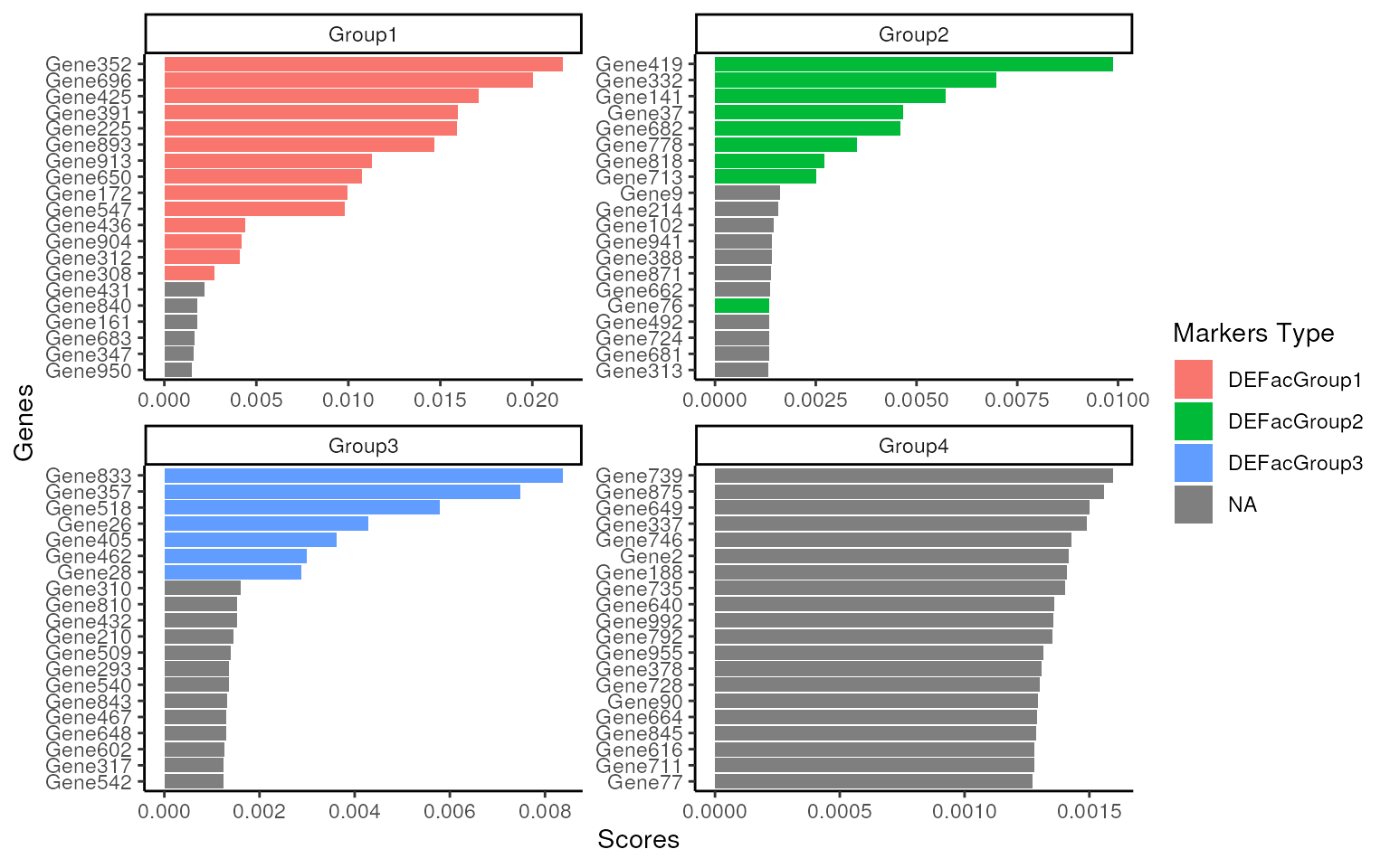
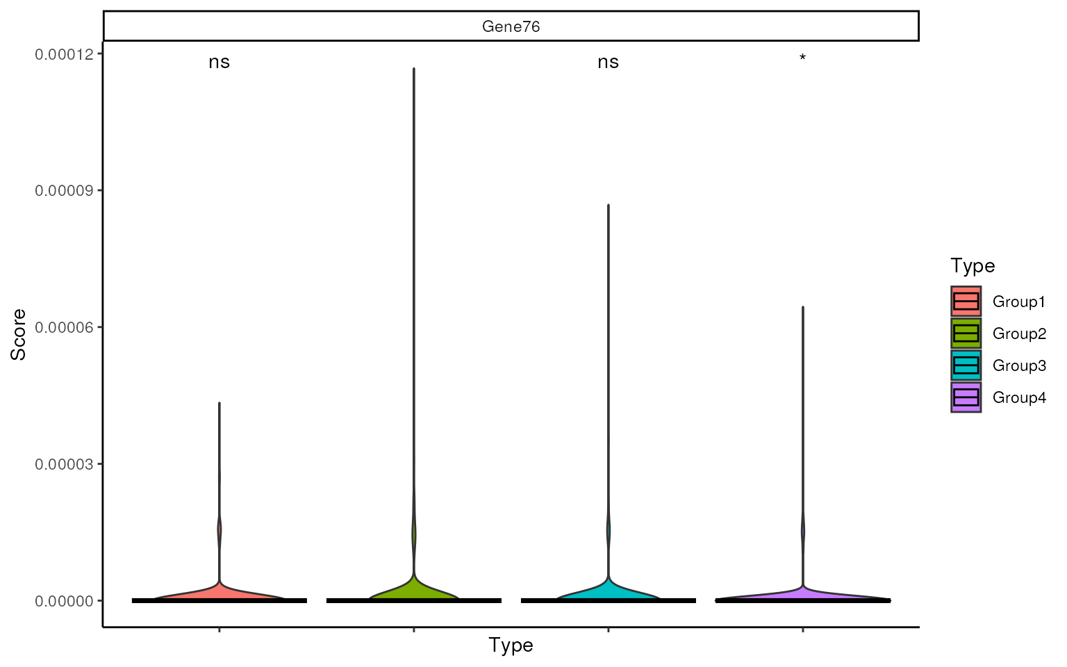
As we can see, there is an UP DEG ‘Gene76’ not popping up in Group 2, we can check the relative expression of this gene using violin plot. It is clear that this gene is not significantly highly expressed in Group 2 and the average expression is quite low across all cells.

This can also be confirmed in data simulation information, where the scale factor is higher in Group2, but the GeneMean is too small to be confident. Thus this gene won’t be selected by smartid.

sin_score_boxplot(
  metadata(data_sim)$tf,
  features = "Gene76",
  ref.group = "Group2",
  label = data_sim$Group
)
#> Warning: `add_rownames()` was deprecated in dplyr 1.0.0.
#> ℹ Please use `tibble::rownames_to_column()` instead.
#> ℹ The deprecated feature was likely used in the smartid package.
#>   Please report the issue at
#>   <https://github.com/DavisLaboratory/smartid/issues>.
#> This warning is displayed once every 8 hours.
#> Call `lifecycle::last_lifecycle_warnings()` to see where this warning was
#> generated.


## sim gene info
SummarizedExperiment::elementMetadata(data_sim)[76, ]
#> DataFrame with 1 row and 8 columns
#>          Gene BaseGeneMean OutlierFactor   GeneMean DEFacGroup1 DEFacGroup2
#>   <character>    <numeric>     <numeric>  <numeric>   <numeric>   <numeric>
#> 1      Gene76   0.00628427             1 0.00628427           1     1.73743
#>   DEFacGroup3 DEFacGroup4
#>     <numeric>   <numeric>
#> 1           1           1

Marker Selection

As we can see from above, there is a distinctly different distribution of feature score between group with DEGs and without DEGs. And there is a clear separation (break point) between the real DEGs and non-DEGs.

To help automatically select real markers for each group, smartid used an expectation maximization (EM) approach to identify which genes fall into the real DEGs distribution and which are not.

Regarding the distribution of scores as a mixture model, here we can choose function markers_mixmdl() in smartid to separate features. There are 2 available mixture model to choose: normal (Gaussian) or gamma. We choose “norm” here as it runs faster.

smartid also allows to plot the mixture distribution plot after EM. It’s obvious that the top 2 components of Group 4 share quite similar distribution, thus no markers will be selected for this group.

set.seed(123)
marker_ls <- markers_mixmdl(
  top_markers = top_m,
  column = ".dot",
  ratio = 2,
  dist = "norm",
  plot = TRUE
)
#> number of iterations= 88
#> `stat_bin()` using `bins = 30`. Pick better value with `binw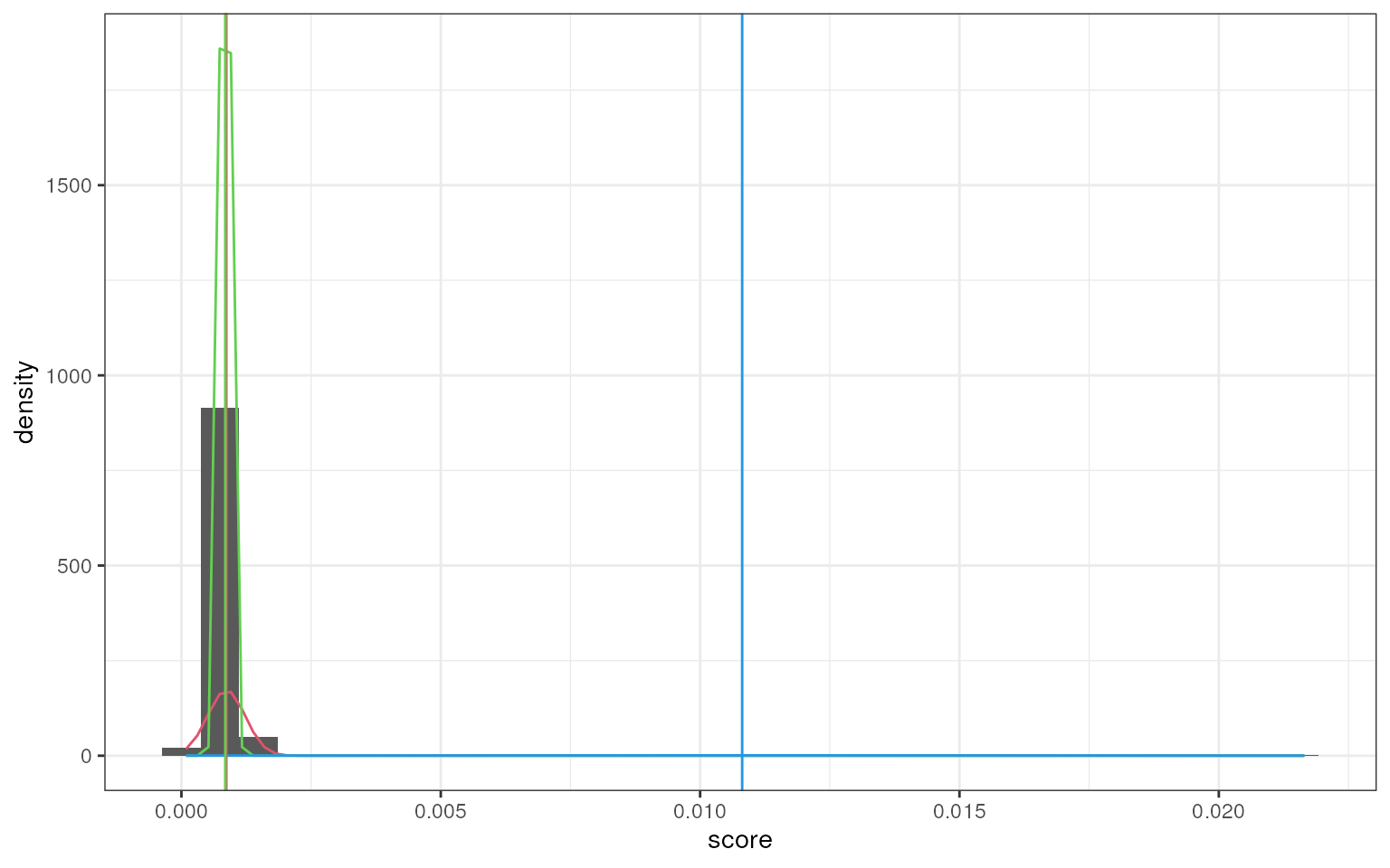idth`.

#> number of iterations= 81
#> `stat_bin()` using `bins = 30`. Pick better value with `binw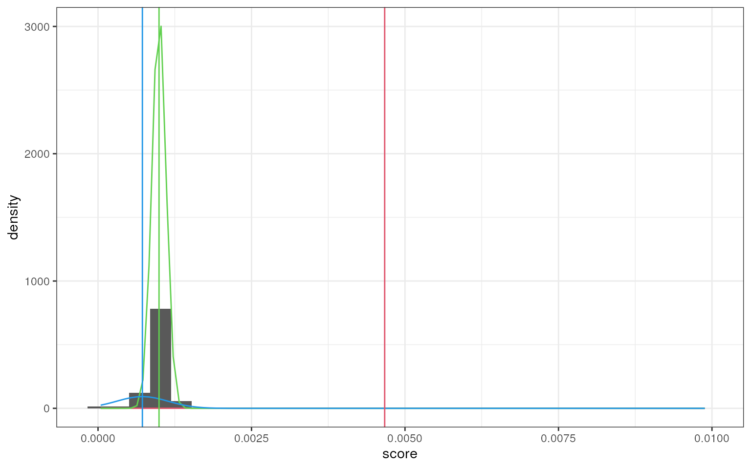idth`.

#> number of iterations= 36
#> `stat_bin()` using `bins = 30`. Pick better value with `binw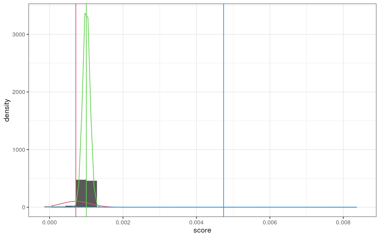idth`.

#> number of iterations= 507
#> `stat_bin()` using `bins = 30`. Pick better value with `binw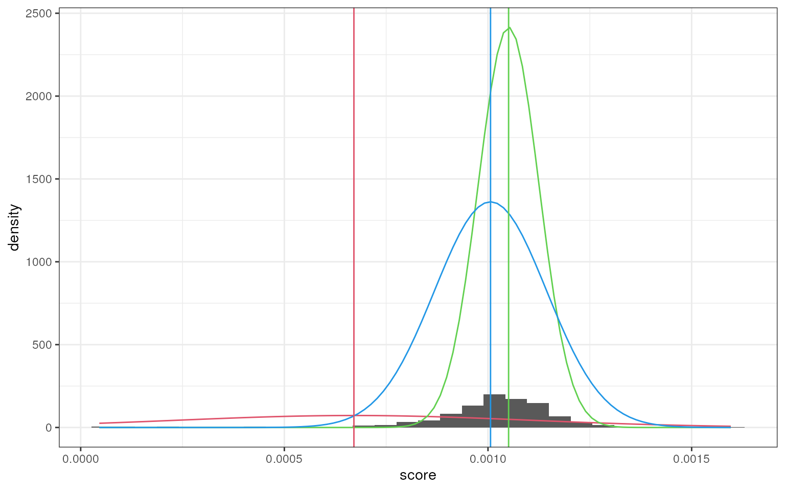idth`.

marker_ls
#> $Group1
#>  [1] "Gene352" "Gene696" "Gene425" "Gene391" "Gene225" "Gene893" "Gene913"
#>  [8] "Gene650" "Gene172" "Gene547" "Gene436" "Gene904" "Gene312" "Gene308"
#> 
#> $Group2
#> [1] "Gene419" "Gene332" "Gene141" "Gene37"  "Gene682" "Gene778" "Gene818"
#> 
#> $Group3
#> [1] "Gene833" "Gene357" "Gene518" "Gene26"  "Gene405" "Gene462" "Gene28" 
#> 
#> $Group4
#> NULL

We can also compare our selected markers with real DEGs. As there is no markers or DEG in group 4, only show overlap from Group1-3. It’s clear that all the markers identified by smartid are real DEGs, with a couple of missing genes in Group 1 and 2. But as what we showed above, those genes only exhibit low mean expression across all cells, thus not confident enough to be selected as markers.

library(UpSetR)

upset(fromList(c(slot(data_sim, "metadata")$up_markers, marker_ls)), nsets = 6)

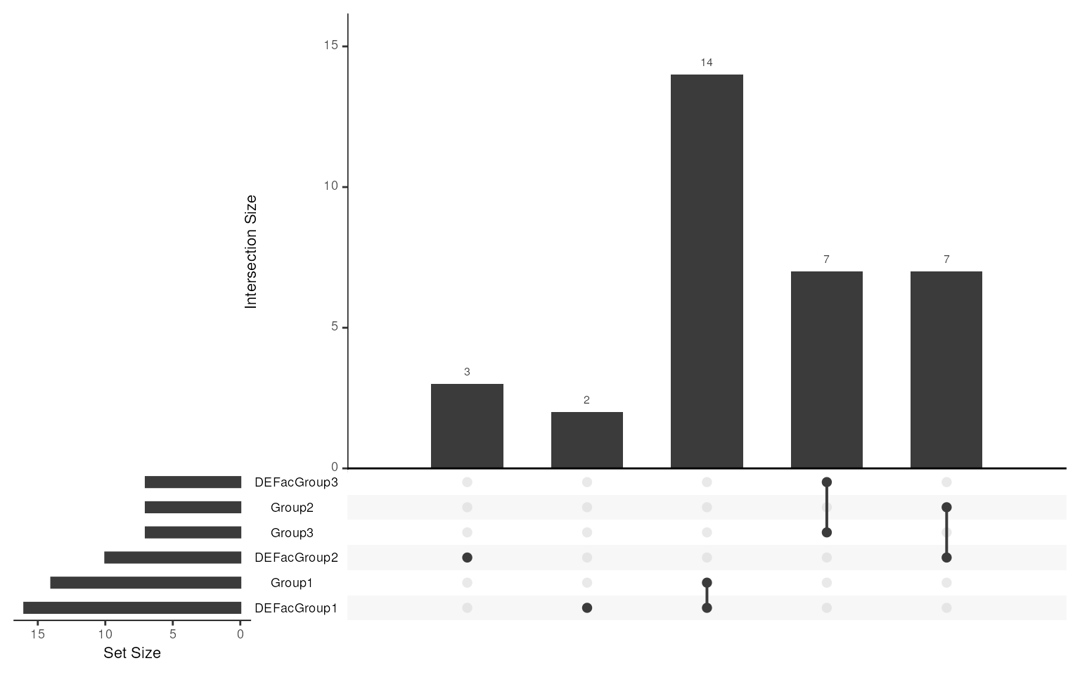
smartid also provides some other implementation of marker selection. Here is another example using mclust. Different from markers_mixmdl(), markers_mclust() doesn’t need a pre-defined number of components (which is default 3 in markers_mixmdl()), instead, it will select the number of components by searching a series of potential numbers. This method is sometimes more robust than markers_mixmdl() but will also take longer running time.

Similarly, this method also allows to plot the mixture distribution for each component, but separately.

set.seed(123)
marker_ls_new <- markers_mclust(
  top_markers = top_m,
  column = ".dot",
  method = "max.one",
  plot = TRUE
)

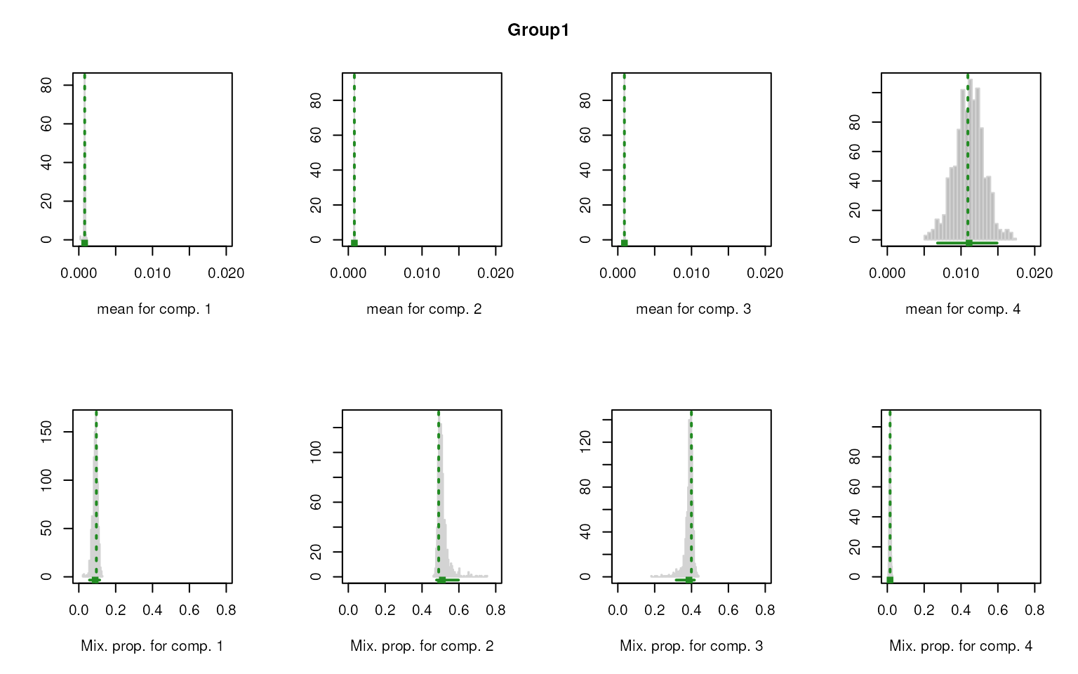
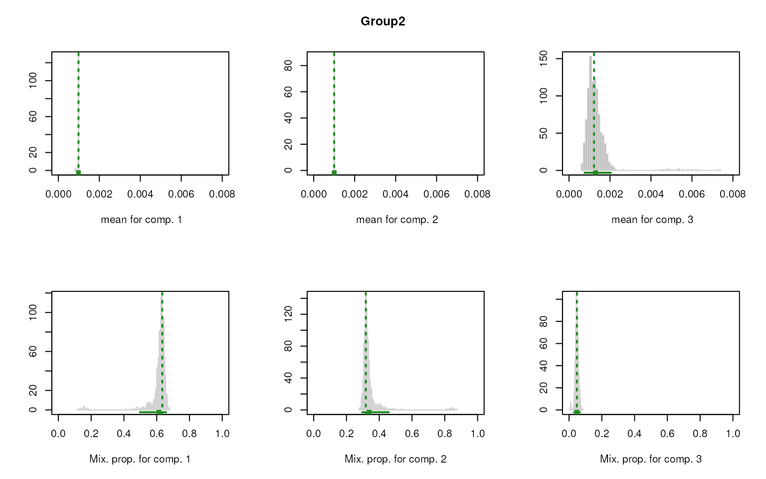
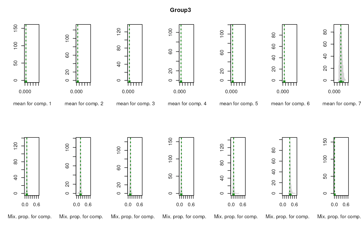
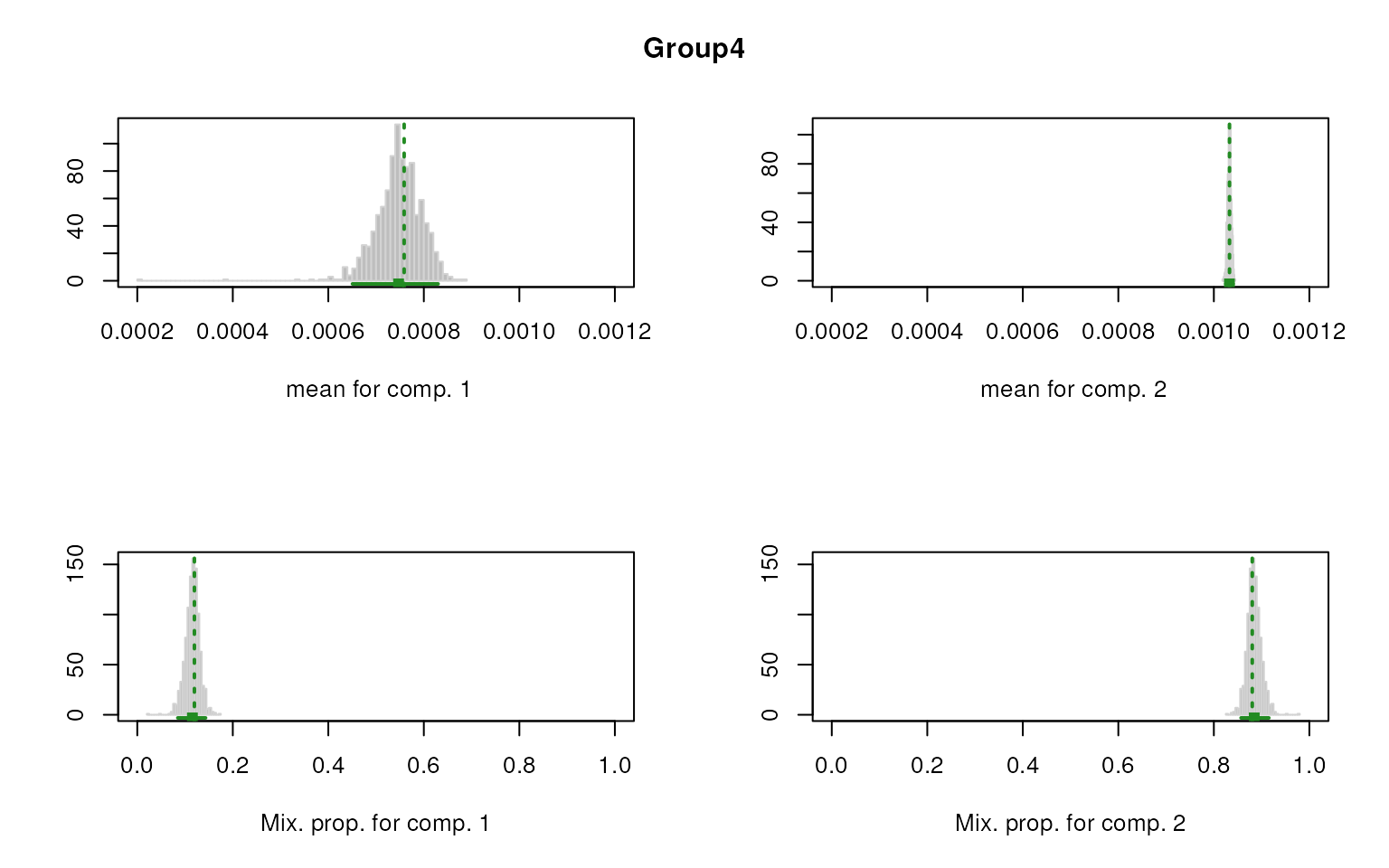
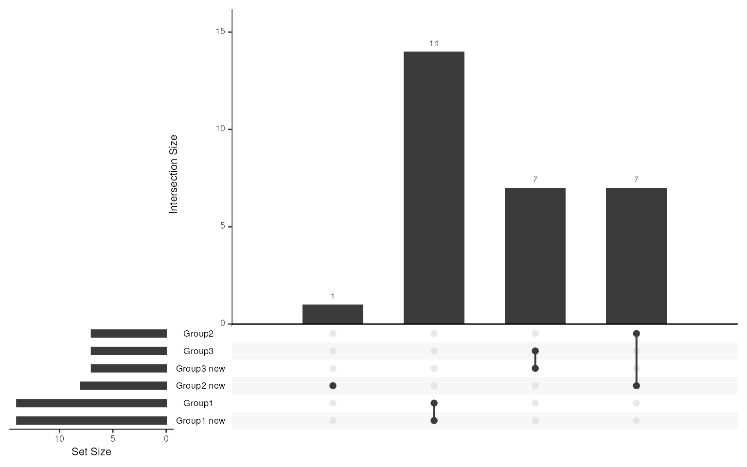
names(marker_ls_new) <- paste(names(marker_ls_new), "new")

We can compare the marker list with the previous one. The overlap result shows 2 methods can achieve almost the same marker list for each group.

upset(fromList(c(marker_ls, marker_ls_new)), nsets = 6)

Un-labeled Data

While for the unlabeled data, smartid also provides the score methods with no need for label information.

Here we choose logTF * IDF_sd * IAE_sd for for gene-set scoring as a use case: $\mathbf{score}=\log \mathbf{TF}*\mathbf{IDF}_{sd}*\mathbf{IAE}_{sd}$

Where IDF and IAE can be termed as: $\mathbf{IDF_i} = \log(1+\mathrm{SD}(\mathbf{TF}_{i})*\frac{n}{n_i+1})$ $\mathbf{IAE_i} = \log(1+\mathrm{SD}(\mathbf{TF}_{i})*\frac{n}{\sum_{j=1}^{n}\hat N_{i,j}+1})$

Score Samples

Similarly, the first step is to score samples/cells using the specified method. This step also starts with raw counts data, without need for data pre-processing, which is quite convenient and fast.

## compute score without label
system.time(
  data_sim <- cal_score(
    data_sim,
    tf = "logtf",
    idf = "sd",
    iae = "sd",
    new.slot = "score_unlabel"
  )
)
#>    user  system elapsed 
#>   0.166   0.032   0.198

## new score is saved and tf,idf,iae all updated
assays(data_sim)
#> List of length 8
#> names(8): BatchCellMeans BaseCellMeans BCV ... counts score score_unlabel
names(metadata(data_sim))
#> [1] "Params"     "up_markers" "tf"         "idf"        "iae"

Compute Overall Score for Gene-set

To compare overall score of the given gene-set, we don’t need to scale and transform score this time. Using gs_score() can easily compute the overall score for each cell based on the given gene-set list.

## compute score for each group marker list
data_sim <- gs_score(
  data = data_sim,
  features = marker_ls[1:3], # group 4 has no markers
  slot = "score_unlabel",
  suffix = "score.unlabel" # specify the suffix of names to save
)

## saved score
colnames(colData(data_sim))
#> [1] "Cell"                 "Batch"                "Group"               
#> [4] "ExpLibSize"           "Group1.score.unlabel" "Group2.score.unlabel"
#> [7] "Group3.score.unlabel"

Now we get 3 columns of score for each group markers. We can then visualize the score across groups, see how well it can discern the target group.

It’s evident that the score can sufficiently separate the target group from all others.

as.data.frame(colData(data_sim)) |>
  tidyr::pivot_longer("Group1.score.unlabel":"Group3.score.unlabel",
    names_to = "group markers",
    values_to = "score"
  ) |>
  ggplot(aes(x = Group, y = score, fill = Group)) +
  geom_boxplot() +
  facet_wrap(~`group markers`, scales = "free") +
  theme_bw()

SessionInfo

sessionInfo()
#> R version 4.4.1 (2024-06-14)
#> Platform: x86_64-pc-linux-gnu
#> Running under: Ubuntu 22.04.5 LTS
#> 
#> Matrix products: default
#> BLAS:   /usr/lib/x86_64-linux-gnu/openblas-pthread/libblas.so.3 
#> LAPACK: /usr/lib/x86_64-linux-gnu/openblas-pthread/libopenblasp-r0.3.20.so;  LAPACK version 3.10.0
#> 
#> locale:
#>  [1] LC_CTYPE=en_US.UTF-8       LC_NUMERIC=C              
#>  [3] LC_TIME=en_US.UTF-8        LC_COLLATE=en_US.UTF-8    
#>  [5] LC_MONETARY=en_US.UTF-8    LC_MESSAGES=en_US.UTF-8   
#>  [7] LC_PAPER=en_US.UTF-8       LC_NAME=C                 
#>  [9] LC_ADDRESS=C               LC_TELEPHONE=C            
#> [11] LC_MEASUREMENT=en_US.UTF-8 LC_IDENTIFICATION=C       
#> 
#> time zone: UTC
#> tzcode source: system (glibc)
#> 
#> attached base packages:
#> [1] stats4    stats     graphics  grDevices utils     datasets  methods  
#> [8] base     
#> 
#> other attached packages:
#>  [1] UpSetR_1.4.0                scater_1.34.0              
#>  [3] scuttle_1.16.0              ggplot2_3.5.1              
#>  [5] splatter_1.30.0             SingleCellExperiment_1.28.1
#>  [7] SummarizedExperiment_1.36.0 Biobase_2.66.0             
#>  [9] GenomicRanges_1.58.0        GenomeInfoDb_1.42.0        
#> [11] IRanges_2.40.0              S4Vectors_0.44.0           
#> [13] BiocGenerics_0.52.0         MatrixGenerics_1.18.0      
#> [15] matrixStats_1.4.1           smartid_1.3.2              
#> [17] BiocStyle_2.34.0           
#> 
#> loaded via a namespace (and not attached):
#>   [1] gridExtra_2.3            rlang_1.1.4              magrittr_2.0.3          
#>   [4] tidytext_0.4.2           compiler_4.4.1           systemfonts_1.1.0       
#>   [7] vctrs_0.6.5              pkgconfig_2.0.3          crayon_1.5.3            
#>  [10] fastmap_1.2.0            backports_1.5.0          XVector_0.46.0          
#>  [13] labeling_0.4.3           utf8_1.2.4               rmarkdown_2.28          
#>  [16] UCSC.utils_1.2.0         ggbeeswarm_0.7.2         ragg_1.3.3              
#>  [19] purrr_1.0.2              xfun_0.48                zlibbioc_1.52.0         
#>  [22] cachem_1.1.0             beachmat_2.22.0          jsonlite_1.8.9          
#>  [25] SnowballC_0.7.1          highr_0.11               DelayedArray_0.32.0     
#>  [28] BiocParallel_1.40.0      broom_1.0.7              irlba_2.3.5.1           
#>  [31] parallel_4.4.1           R6_2.5.1                 bslib_0.8.0             
#>  [34] stringi_1.8.4            car_3.1-3                jquerylib_0.1.4         
#>  [37] Rcpp_1.0.13              bookdown_0.41            knitr_1.48              
#>  [40] mixtools_2.0.0           splines_4.4.1            Matrix_1.7-1            
#>  [43] tidyselect_1.2.1         abind_1.4-8              yaml_2.3.10             
#>  [46] viridis_0.6.5            codetools_0.2-20         plyr_1.8.9              
#>  [49] lattice_0.22-6           tibble_3.2.1             withr_3.0.2             
#>  [52] evaluate_1.0.1           survival_3.7-0           desc_1.4.3              
#>  [55] mclust_6.1.1             kernlab_0.9-33           pillar_1.9.0            
#>  [58] BiocManager_1.30.25      ggpubr_0.6.0             carData_3.0-5           
#>  [61] janeaustenr_1.0.0        checkmate_2.3.2          plotly_4.10.4           
#>  [64] generics_0.1.3           sparseMatrixStats_1.18.0 munsell_0.5.1           
#>  [67] scales_1.3.0             glue_1.8.0               lazyeval_0.2.2          
#>  [70] tools_4.4.1              data.table_1.16.2        BiocNeighbors_2.0.0     
#>  [73] tokenizers_0.3.0         ScaledMatrix_1.14.0      ggsignif_0.6.4          
#>  [76] locfit_1.5-9.10          fs_1.6.4                 grid_4.4.1              
#>  [79] tidyr_1.3.1              colorspace_2.1-1         nlme_3.1-166            
#>  [82] GenomeInfoDbData_1.2.13  beeswarm_0.4.0           BiocSingular_1.22.0     
#>  [85] vipor_0.4.7              Formula_1.2-5            cli_3.6.3               
#>  [88] rsvd_1.0.5               textshaping_0.4.0        fansi_1.0.6             
#>  [91] segmented_2.1-3          S4Arrays_1.6.0           viridisLite_0.4.2       
#>  [94] dplyr_1.1.4              gtable_0.3.6             rstatix_0.7.2           
#>  [97] sass_0.4.9               digest_0.6.37            SparseArray_1.6.0       
#> [100] ggrepel_0.9.6            htmlwidgets_1.6.4        farver_2.1.2            
#> [103] htmltools_0.5.8.1        pkgdown_2.1.1            lifecycle_1.0.4         
#> [106] httr_1.4.7               MASS_7.3-61

Jinjin Chen

13 Nov 2024

Introduction

Installation

Prepare Data

Labeled Data

Score Samples

Scale and Transform Score

Marker Selection

Un-labeled Data

Score Samples

Compute Overall Score for Gene-set

SessionInfo